Instances: SREF and AREF

A SREF is a single instance of a cell placed at (x, y) with rotation / magnification / reflection. An AREF is a rectangular array of instances (rows × cols with separate column and row step vectors).

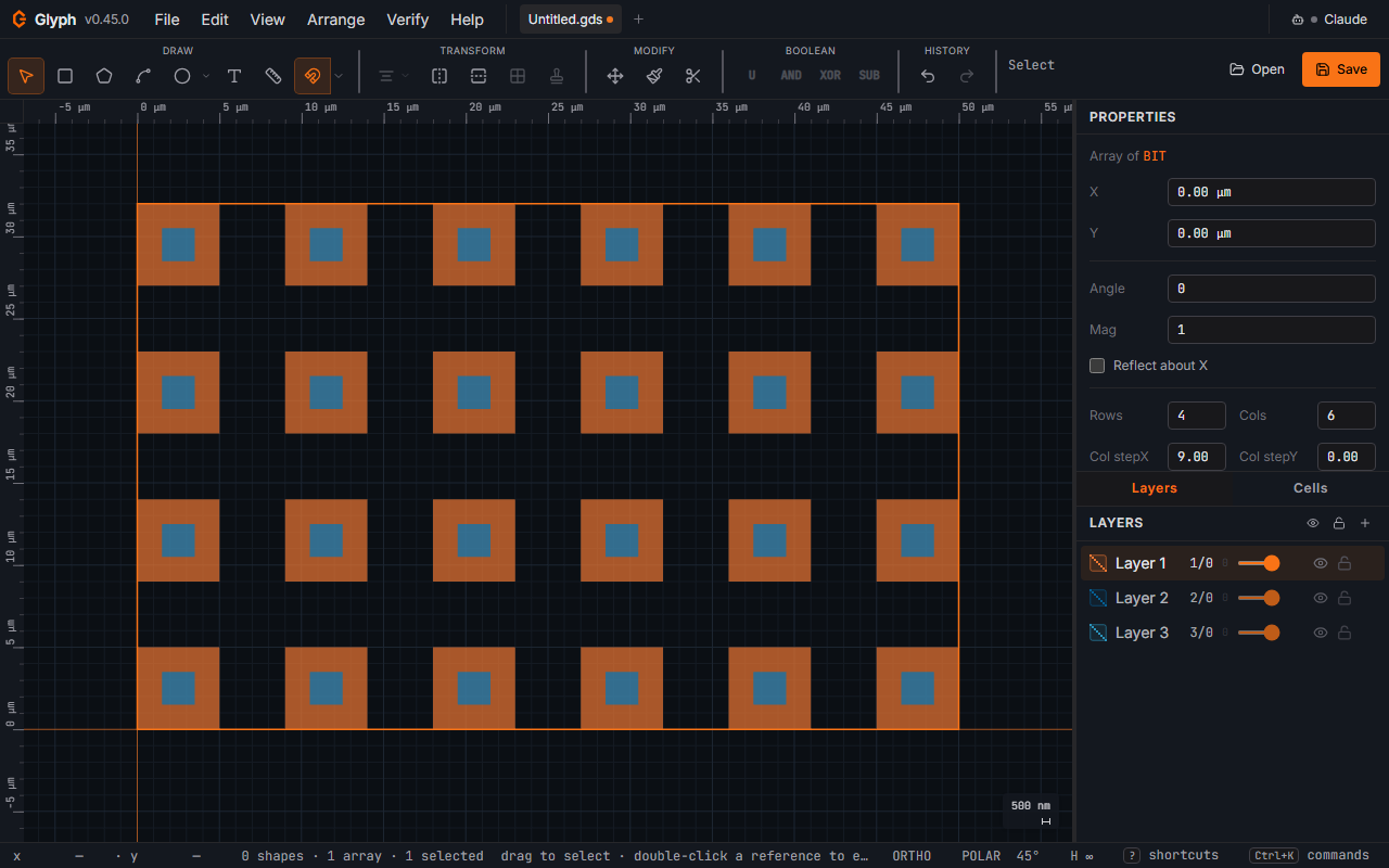Swipe →View full image

Inserting an SREF

1. In the Cells panel, click the "Insert Instance" icon on the target cell.
2. Enter rotation / magnification / reflect in the dialog.
3. Click on the canvas to place.
4. Rotation etc. can be edited later in the Properties panel when the SREF is selected.

Inserting an AREF

1. In the Cells panel, click the "Insert Array" icon on the target cell.
2. Fill in rows, cols, and the col-step / row-step vectors (nm per column and nm per row).
3. Click on the canvas to place the origin.
4. All array parameters can be edited later in the Properties panel.

Arraying an instance you already placed. Select the SREF and choose Arrange → Array…: with exactly one instance selected (and no shapes) it opens the Insert-array dialog directly, already filled in from that instance (its cell, rotation, magnification and reflection, with a step sized to its placed extent), and the array's origin is the instance's own position — there is no canvas click. Replace the selected instance is on by default, so the instance becomes the array's first element instead of staying underneath it; untick it to keep the instance and add the array beside it. Either way it is one undo step, and undo puts the instance back exactly where it was.

Refs are selected and moved just like shapes. Selection colors: accent (orange) for shapes, amber for refs.

External symbol library (Cells panel → Library)

The Library section at the bottom of the Cells panel opens another design file (any format Glyph can open — GDS, OASIS, CIF, DXF, DWG, SVG) as a read-only reference library — the DTU-style "keep a facility's mark set in one file, drop symbols from it into any design" workflow. It is not a live link: the file is parsed once into a detached copy that Glyph holds only for this session (never autosaved, never a tab of its own), and clicking a cell in its list copies that cell — plus anything it references — into your document and arms the same placement ghost an ordinary SREF insert uses. The next click on the canvas drops one instance and the ghost is gone, as with any SREF insert; to drop another, arm it again (the copied cell's Insert cell instance (SREF) icon in the Cells panel, or click the library cell again, which reuses the copy it already made). There is no size cap on what a single click copies in — a symbol whose subtree holds a large nested hierarchy comes in whole. The import happens on the click itself, before you place anything — pressing Esc cancels the armed placement ghost but does not undo the copy: the imported cell stays in your document as its own undo entry, so Ctrl+Z (not Esc) is what removes it.

Placing the same symbol twice, or two symbols that share a nested cell, doesn't duplicate the shared geometry: Glyph recognizes a cell it has already copied in from this library (by filename + original name) and reuses it. That recognition lasts for the session (and survives autosave recovery), but the provenance note is not written into a saved .gds — after you save, close and reopen the design, placing the same symbol again imports a fresh copy (renamed, with a toast) instead of reusing the old one. If a symbol's name collides with something already in your document, the copy is renamed (NAME_1, NAME_2, …) and a toast says so. If the placed symbol's subtree contains a reference to a cell that was never actually defined in the library file, the reference is kept dangling under a name that can't collide with anything already in your document, or with any name the library itself uses — renamed with a _1, _2, … suffix just like a real cell would be — and a toast names the missing symbol (and the parked name too, if it was renamed). If a cell with that exact name is later added — by you, or by placing another symbol from the same library — the dangling reference will then bind to it, by name, the same as any GDS reference. Recently opened libraries are remembered (browser permitting) for one-click reopening. Closing the library only closes the reference list — cells already placed stay exactly as they are.

Component library (parametric cells)

View → Component library — or the library icon at the end of the toolbar's Draw group — opens a dock on the left edge with several libraries, chosen from the dropdown at its top:

• Standard cells — parametric fab marks: alignment cross, Greek cross (van der Pauw), a true dual-scale overlay vernier, box-in-box, a keyed alignment cross (an off-axis tab breaks the plain cross's rotational/mirror symmetry, so a mask loaded rotated or mirrored is never mistaken for a correctly-oriented one — the tab can ride its own layer), die frame, line/space grating, bond-pad array.
• Metrology marks (single-layer) — process-control & metrology structures, each drawn entirely on the one active layer: Siemens star and USAF-1951 three-bar resolution targets (correct 2^(1/6) pitch step and 5:1 bar aspect), a CD/dose step wedge, a four-terminal Kelvin cross, a TLM ladder, a via/contact chain, an interdigitated leakage comb, a cross-in-box alignment fiducial, a seal ring, corner crop marks, a dummy-fill tile, and a Code 128 barcode (Code Set B — text, module width, bar height, and an optional human-readable label centred under the bars; only the bars are drawn, so keep at least 10 modules clear of other features on each side — the standard quiet zone). The barcode's Text is a plain text field in the Properties panel (and in the parameters shown while the barcode is armed for placement): Enter or clicking away applies it as one undo step, Esc abandons it. Text the barcode cannot encode is refused rather than silently changed — a character outside printable ASCII (space through ~), empty text, or more than 48 characters leaves the field outlined in red with the reason underneath, and nothing is applied until you fix it. A Data Matrix (ECC 200) 2D code sits beside it: square symbols from 10×10 to 48×48 modules, or with Symbol shape set to Rectangular or Auto the six rectangular sizes 8×18 to 16×48 for a thin scribe lane, chosen as the smallest that holds the text (or set Min symbol size to keep a batch of IDs the same size), with a Module size length and adjacent dark modules drawn as one merged polygon rather than a box per module. Its Text takes any ASCII character (0–127, tabs and control characters included) and is refused the same way past 174 characters — digits pair up, so up to 348 digits fit. Only the dark modules are drawn, so keep at least one module clear around the symbol, or tick Reverse contrast to draw the light modules plus a solid frame Quiet zone (reverse only) modules wide instead, for a process where drawn features read bright.
• Microfluidics — channels (straight / serpentine / spiral / taper), inlet-outlet ports, reservoirs, observation chambers, junctions (T / Y / cross), a flow resistor, mixers (serpentine / staggered-herringbone with the correct asymmetric grooves, optionally on its own second-etch groove layer / split-and-recombine / Y / a rotary peristaltic mixer with three control-line valves), a pillar array (DLD with a fractional row-shift ε / filter), a weir gap filter, a cell-culture chamber, a Christmas-tree gradient generator, a cell-trap array, a Tesla fluidic-diode valve, a capillary burst valve, a Quake-style crossing membrane valve (flow + control layers), and droplet structures (T-junction, flow-focusing, and a parking array).
• Passive photonics — silicon-photonics building blocks on one waveguide-core layer: straight waveguides, Euler bends, S-bends, spot-size tapers, waveguide crossings, directional couplers, MMI 1×2 / 2×2 splitters, Y-branches, ring and racetrack resonators, an add-drop ring (a ring between a through bus and a drop bus, each with its own gap), a sidewall Bragg grating (period, fill factor, corrugation and period count), grating couplers, an edge (butt) coupler, and spiral delay lines. Parts expose optical ports, so the Connect ports router works here too.
• Diffractive optics — single-layer (binary) diffractive elements: Fresnel zone plate, spiral/vortex zone plate, photon sieve, Dammann fan-out grating, and a diffractive (Fresnel) microlens array.
• MEMS — a comb-drive electrostatic actuator (interdigitated stator/rotor finger combs on a two-beam cantilever suspension with anchor pads), a folded-beam (Tang-style) flexure spring (two anchors, outer/inner trusses and parallel beams guiding a shuttle in a straight line, with ports at the shuttle's two ends so a comb drive can be positioned collinear with it), a perforated proof mass (a square or offset-row release-hole lattice, drawn as hole-free abutting bars — reads the max release undercut as a derived number), and a cantilever array (N beams of linear or geometric swept length off a shared anchor — the standard stiction / residual-stress test ladder, with optional length labels and a movable anchor layer). All single-layer except the cantilever array's optional anchor layer.
• Overlay & PCM (multi-layer) — process-control structures that measure one layer against another, so each maps its extra layers before you place it (see Multi-layer components below): a bar-in-bar overlay target (four reference bars on the previous layer, four on the current one, with an optional programmed offset for building a calibration array), a two-layer vernier in X and Y with a coarse pair for capture and a fine pair for the reading (resolution = the pitch difference, 200 nm by default), a cross-in-window alignment pair (mask-side cross, wafer-side clear window), a van der Pauw Greek cross with contact windows and probe pads (sheet resistance = π/ln2 × the measured resistance), a meander sheet resistor whose squares count is corner-corrected at 0.56 per turn and can be drawn on the mask as a label, a four-terminal Kelvin via chain whose links alternate between the lower and upper metal so every via is measured, and a two-layer registration mark (tick + key) — a coarse tick-ladder scale inside a four-corner bracket frame on the active layer (the level being aligned), plus a four-way interlocking staircase key on the fine role layer (map it to the reference level already on the wafer), modelled on a real CleWin export's alignment-mark idiom, and a 3-layer nested cross mark whose arm width steps up in three tiers (1×/3×/5× a base stroke) with the mid and outer role layers each filling the notch left at one step — correctly registered the three levels tile solid, so one mark tracks overlay across three process levels (e.g. poly/contact/metal-1) instead of needing three separate 2-layer targets, and a 3-layer comb overlay target — three interdigitated combs, one per layer, at a deliberately mismatched pitch between the active layer and the mid/upper role layers, so misregistration reads as reduced tooth overlap area rather than a coinciding tick: every comb keeps one tooth exactly on the mark's centreline, so a correctly registered target shows all three centre teeth coinciding while every other tooth pair drifts apart with distance from centre. Defaults follow the standard characterization literature (van der Pauw 1958; Buehler & Thurber 1978; Hall 1967; Proctor & Linholm 1982; Schroder, Semiconductor Material and Device Characterization).
• Marks & targets — ready-made fixed-size fab marks, each placed as an instance of its own generated cell: alignment cross, L-mark, bullseye (box-in-box), vernier scale, fiducial, die frame, dicing scribe lane, and orientation arrow. Click a card, then click the canvas to drop it; the card stays armed, so each further click drops another mark, until Esc, a right-click, a tool switch or a switch to another tab.

Each component shows a live thumbnail. Drag a card onto the canvas to drop it at the cursor, or click a card then click the canvas to place it. A placed component is a normal cell + instance, so it moves, rotates, copies, and exports to GDS like anything else. If this is the very first thing you place into an otherwise-empty cell and it is not comfortably in view — bigger than the view in both directions (e.g. a default-sized channel dropped at the default zoom), far smaller than it, or running past an edge — Glyph zooms to fit it automatically and says so in a toast — Ctrl+0 still zooms to fit on demand any time after that.

Connect ports. For libraries whose parts have connection ports (Microfluidics and Passive photonics), a Connect ports button appears under the library dropdown — also in Arrange → Connect ports and in the command palette (Ctrl+K) by that name, both of which open the dock for you if it isn't already. Click it, then click one component's port and another's, to route a channel between them. The connector stays attached: move or rotate either component, or edit its parameters, and it re-routes automatically. Select it and toggle Tangent in the Properties panel for a smooth curve that leaves and enters along each port's direction (with a Bend control), or turn it off for a straight run; its width follows the channel it joins, and it is drawn on the layer of the component you start from (the active layer only when neither end is a port); if the two components sit on different layers, a warning says the route took the first one's. Re-mapping a component's layer role in Properties moves a route that sits on that role's layer along with it, in the same undo step; a route you moved to another layer yourself stays where you put it. If a component was saved before a Glyph update moved its ports, its routes keep the ends they were saved with and a warning names the component; editing any of its parameters regenerates it, and the routes then move to its current ports. An end clicked away from any port is a free point with no direction of its own, so the route ends there without looping past it. Esc cancels mid-route. On GDS export the connector is written as an ordinary path (the live link is app-only). Every port also carries a domain (optical for Passive photonics, fluidic for Microfluidics — flow and control channels alike); connecting two ports of different domains still routes the channel, but shows a warning toast, since that combination is usually a mistake (a control line landing on a flow port) though occasionally a deliberate off-chip bridge.

Export connectivity (File → Export ▸ Export connectivity…). Writes the design's port↔port connectivity graph as JSON — which component instances are placed, their named ports, and how the connectors on the canvas join them. This is a hub, not a suite: Glyph performs no simulation or valve-sequence generation itself, but the graph is the same shape a MINT/Fluigi-class microfluidics-connectivity tool (or any other downstream consumer) needs as input, so a chip's connectivity can be handed off without redrawing it. The file is versioned (schemaVersion) and every id is stable (SREF ids, port ids, a synthesised id for a free-standing junction where two connectors simply meet, and an explicit kind: 'dangling' node — never a silent drop — for a connector end that no longer resolves to a live component) — see src/model/connectivity.ts for the exact shape if you're writing a consumer.

Configure before you place. When you click a card to arm click-to-place, a ghost follows the cursor and the Properties panel shows that component's parameters — set them before dropping, and the ghost updates live. While the ghost is armed you can also rotate it with [ / ] (∓90°, hold Shift for ∓45°) or R (90° clockwise) and mirror it with F; the orientation carries into the drop. The ghost stays armed after each drop, so every further click places another copy (each its own undo step, the newest one selected); Esc, a right-click, switching tools or switching to another tab (or opening a file into this one) finishes. The banner says so: "Click to place, Esc to finish". An instance placed from the Cells panel (Insert instance / Insert array) is placed once and disarms. The library remembers the last parameters you used for each component, so re-placing a part keeps your settings (within the session) — it also remembers which library you last had selected, so closing and reopening the dock returns you to it instead of resetting to Standard cells. A banner at the top of the canvas names the component you are placing. Select a placed component and Properties lists its parameters first, then its read-only Ports (each port's world position on one line, its outward angle and type on the next).

Snap on place. The ghost is magnetic — its anchor latches onto nearby existing geometry (vertices, edges, and aligned coordinates), with pink guide lines showing the alignment, and the grid as the fallback. So you can drop a fiducial exactly on a die corner or align a test structure to an existing feature without eyeballing it. (Microfluidic components additionally snap their ports to mating channels, which takes priority.)

Multi-layer components. Most components draw on the active layer alone. Some need more than one: the thermo-optic phase shifter in Passive photonics, the keyed alignment cross in Standard cells (its key tab can move to its own inspection layer), the Quake valve / rotary mixer / herringbone mixer in Microfluidics, and every component in Overlay & PCM (multi-layer) (an overlay target that measured only one layer would measure nothing — up to three extra layers there, e.g. the via chain's via, upper metal and pad levels). When you arm one of these, the Properties panel shows a Layers section with one picker per role; set them before you click the canvas. Roles you leave alone default to the active layer, so the component still appears (just not fabricable). The mapping is stored with the placed component, so editing its parameters later regenerates every part onto the layer you chose.

Resize by parameter. Select a placed component and edit its parameters (channel width, length, turn count, pillar pitch, …) in the Properties panel — each field shows its valid range, and a Reset link restores the defaults. The geometry regenerates on each change as a single undo step. If a parameter conflicts with another (e.g. an overlap longer than the part it sits on), Glyph clamps it automatically and shows an amber "Adjusted to …" note next to the affected field — the canvas always reflects the adjusted value, never the typed one. Parameters live with the document and survive autosave; a .gds export keeps the geometry as polygons but not the parametric link (the same way text and letterSpacing are flattened on export).